Semimajor Axis Survey and Residuals
Distribution
The results of a semimajor axis survey with
m
2
= 10 M
J
line is the unweighted least squares fit to 440
orbits, with slope b=1.74 ± 0.03 and intercept
a=1.30 ± 0.03 (all quoted errors are 1
formal
uncertainties). The standard deviation of the
residuals is
= 0.41. Agreement with the LFM
values for orbits interior to Jupiter (b=1.73 ±
0.19, a=1.53 ± 0.34) is well within the formal
uncertainties. This agreement illustrates the
apparent robustness of the relation. It appears
that a and b are insensitive to the mass ratio for
this dynamical configuration.
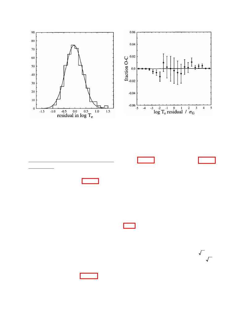
The distribution of the data points in log T
e
from the least squares fit (i.e., the residuals) is
approximately Gaussian. Figure 4 is a histo-
gram of the distance in log T
e
from the solid
line in Figure 3. The smooth curve in Figure 4
is the best-fit Gaussian to the histogram data.
It was found that the best fit is achieved by
excluding the "bump" in the right-hand tail
(represented by four orbits near 1.4). With
standard deviation and mean as free parame-
ters, we find
µ
=-0.039 and
G
=0.39, which is
reassuringly close to the RMS deviation,
=
0.41. A more quantitative view of the fit of the
histogram data to a Gaussian is shown in Fig-
ure 5. Here we show the difference between
the observed and expected fraction of data
points falling into the histogram bins. The
error bars are ±1
and represent the error in
the fraction, which is proportional to
(and
n
not the fractional error, which goes as
).
1/ n
The abscissa is the residual in units of
G
.
There are no significant deviations, including
the points in the tail that were excluded in the
Chaotic Motion in the Outer Asteroid Belt
page 11
Figure 4.
Histogram of the difference of log T
e
(ob-
served event time) from the linear fit to the semimajor
axis survey data (solid line) of Figure 3. Smooth curve
is the best-fit Gaussian, with
G
=0.39.
Figure 5.
Difference between observed and expected
fraction of data points falling into histogram bins of
Figure 4, for a Gaussian distribution. Error bars are
±1
.