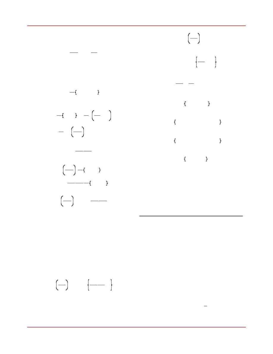
Suppose we have a scalar function of
M parame-
ters,
. Then the variation of
f is
f (p
1
,
¬, p
M
)
(16)
Df
=
S
k
=
1
M
¹f
¹p
k
Dp
k
h ¹f
¹p
$ Dp
Now suppose
N measurements of the parameters
are taken and then the function
f computed from
p
these observationally determined parameters. The
variance of
f is then
(17)
r
f
2
=
1
N
(
f
i
-
Ó f Ô)
2
i
Approximate
by from (16). Then
f
i
-
Ó f Ô
Df
(18)
r
f
2
=
1
N
(
Df )
2
i
=
1
N
¹f
¹p
$ Dp
2
i
=
1
N
S
k
=
1
M
¹f
¹p
k
2
Dp
k
2
+
S
j, k
j
!k
¹f
¹p
j
¹f
¹p
k
Dp
j
Dp
k
i
=
S
k
¹f
¹p
k
2
1
N
(
Dp
k
)
2
i
+
S
j, k
j
!k
¹f
¹p
j
¹f
¹p
k
1
N Dp
j
Dp
k i
h
S
k
¹f
¹p
k
2
r
k
2
+
S
j, k
j
!k
¹f
¹p
j
¹f
¹p
k
r
jk
2
If the observations are uncorrelated, the cross terms
(double sum) tend to cancel. Equation (18) describes
the propagation of errors.
Now consider our least squares parameter esti-
mation, eq. (13). The parameters are quantities de-
a
termined from
N measurements,
, with
[
y
i
]
corresponding measurement errors
.
In light of
r
i
(18), and with a slight abuse of vector notation, we
may write the parameter variance as
(19)
r
a
2
=
¹a
¹y
i
2
r
i
2
i
+
¹a
¹y
i
¹a
¹y
j
r
ij
2
j
i
We will assume that the observational errors are
individually uncorrelated,
. Then we
r
ij
=
0
¼ i ! j
are left with
(20)
r
a
2
=
¹a
¹y
i
2
r
i
2
i
Now, from (13) and (8) we have
(21)
a
=
C $ S
=
C $
y
i
r
i
Z(t
i
)
i
Thus,
(22)
¹a
¹y
i
=
1
r
i
C $ Z(t
i
)
Hence, (20) becomes
(23)
r
a
2
=
(
C $ Z(t
i
))
2
i
The k
th
component of (23) may be written
(24)
r
a
k
2
=
[
C $ Z(t
i
)]
k
[
C $ Z(t
i
)]
k i
Since is symmetric,
C
(25)
r
a
k
2
=
[
C $ Z(t
i
)]
k
[
Z(t
i
)
$ C]
k i
Interchange the order of summations:
(26)
r
a
k
2
=
[
C $ Z(t
i
)
Z(t
i
)
i
$ C]
kk
Using (9), we have
(27)
r
a
k
2
=
[
C $ A $ C]
kk
=
[
C $ C
-
1
$ C]
kk
=
[
C]
kk
which completes the derivation of (14).
3.4. Nonlinear Parameter Estimation.
Consider the condition equations (5). If the
model function
is nonlinear in the parameters
y(t, a)
, then the simple separation, eq. (6), which led to
a
the easily-solved normal equations, (12), is no longer
possible. Our goal is to minimize (4) with respect to
variation of the model parameters, despite the nonlin-
ear dependence of the model function on the parame-
ters. To do this, we will adopt an iterative approach.
Let
, where are the true (or, more accu-
a h a~
+
Da
a~
rately, best) values of the parameters. Assume we
start with parameter values that are close to the best
values. We can then approximate (4) with a trun-
cated Taylor series:
(28)
x
2
(
a) l x
2
(
a~)
-
Da $ B
+
1
2
Da $ M $ Da
where
Chapter 3: Parameter Adjustment
D:\Newcomb\Documentation\NewcombManual.lwp
11 of 19
10:42pm April 23, 1997
