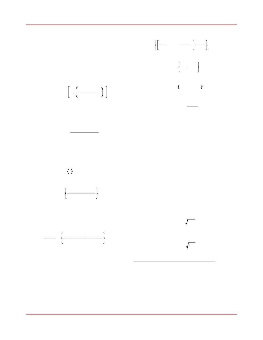
assumed to have two components -- systematic
errors and random errors. We assume the systematic
components are modeled with bias parameters, which
will be estimated. It is the random components
which we assume to be uncorrelated and normally
distributed. Hence, the probability of a specific data-
set occurring, given a model with
n physical and bias
parameters (a vector of length
n), is the product of
a
the probabilities of the
N individual data points:
(1)
P i
P
i
=
1
N
exp
-
1
2
y
i
-
y(t
i
,
a)
r
i
2
where
y
i
are the data and
is the model
y(t
i
,
a)
function. Maximizing the probability means mini-
mizing the negative of the logarithm of this expres-
sion, which within a factor of two becomes
(2)
x
2
h
S
i
=
1
N
[
y
i
-
y(t
i
,
a)]
2
r
i
2
We recognize minimization of (2) as being
equivalent to minimizing chi-squared, the usual least
squares method. For notational convenience, intro-
duce the summation operator
(3)
$
i
h
S
i
=
1
N
(
$)
Thus, (2) is
(4)
x
2
=
[
y
i
-
y(t
i
,
a)]
2
r
i
2
i
When this operator is used, summation is always
over the
N observational data points.
Minimization of (4) requires the set of
n
equations
(5)
-
1
2
¹x
2
¹a
=
y
i
-
y(t
i
,
a)
r
i
¹y(t
i
,
a)
r
i
¹a
i
=
0
to be satisfied simultaneously. Let the model
function have the generalized representation
(6)
y(t, a)
=
S
k
=
1
n
a
k
Y
k
(
t) h a $ Y(t)
where the
Y
k
(t)
are functions of time and the vector
. The basis functions
Y
(
t
)
h [Y
1
(
t
)
,
Y
2
(
t
)
,
¬, Y
n
(
t
)
]
are not restricted to linearity and may have any
Y
k
(
t)
form (polynomials, trig functions, etc.). The linearity
that is important is in the dependence of the model
function on the parameters
.
Then (5) becomes
a
(7)
y
i
r
i
-
S
k
=
1
n
a
k
Y
k
(
t
i
)
r
i
Y(t
i
)
r
i
i
=
0
Define the vector
(8)
S h
y
i
r
i
Z(t
i
)
i
and the symmetric matrix
(9)
A
jk
h Z
j
(
t
i
)
Z
k
(
t
i
)
i
where, for convenience, we have set
(10)
Z(t
i
)
h Y
(
t
i
)
r
i
Then (7) becomes
(11)
S
k
=
1
n
A
jk
a
k
=
S
j
or
(12)
A $ a
=
S
Hence, the parameters are determined from the solu-
tion vector
(13)
a
=
A
-
1
$ S
Equations (12) are the
normal equations. The
matrix
is the
covariance matrix. The covari-
C h A
-
1
ance matrix is the key to
formal knowledge of the er-
rors in the parameter estimates, as well as the
correlations between the various parameters. Indeed,
as we shall see in the next section, the parameter er-
rors are the diagonal elements of ,
C
(14)
r
k
h C
kk
The off-diagonal elements are the cross correla-
tions,
(15)
r
jk
h C
jk
3.3. Formal Parameter Errors.
This section contains a derivation of (14). We
begin with a statement of propagation of errors,
which we then use to define the formal errors of the
parameters. Using the definition (9), we then arrive
at (14).
Chapter 3: Parameter Adjustment
D:\Newcomb\Documentation\NewcombManual.lwp
10 of 19
10:42pm April 23, 1997
