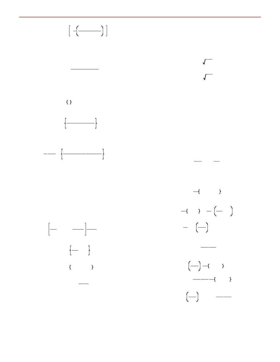
(1)
P i
P
i
=
1
N
exp
-
1
2
y
i
-
y(t
i
, a)
r
i
2
where the y
i
are the data and
is the model function.
y(t
i
, a)
Maximizing the probability means minimizing the negative of
the logarithm of this expression, which within a factor of two
becomes simply
(2)
x
2
h
S
i
=
1
N
[y
i
-
y(t
i
, a)]
2
r
i
2
We recognize minimization of (2) as being equivalent to
minimizing chi-squared, the usual linear least squares method.
For notational convenience, define the summation operator
(3)
$
i
h
S
i
=
1
N
(
$)
Thus, (2) can be written
(4)
x
2
=
[y
i
-
y(t
i
, a)]
2
r
i
2
i
When this operator is used, summation is always over the N
observational data points.
Minimization of (4) requires the set of equations
n
(5)
-
1
2
¹x
2
¹a
=
y
i
-
y(t
i
, a)
r
i
¹y(t
i
, a)
r
i
¹a
i
=
0
to be satisfied simultaneously. Let the model function have the
generalized representation
(6)
y(t, a)
=
S
k
=
1
n
a
k
Y
k
(t) h a $ Y(t)
where the
are functions of time and the vector
Y
k
(t)
. The basis functions
are not
Y
(
t
)
h [Y
1
(
t
)
, Y
2
(
t
)
,
¬, Y
n
(
t
)
]
Y
k
(t)
restricted to linearity and may have any form (polynomials,
transcendental functions, etc.). The linearity that is important
is in the dependence of the model function on the parameters
Equation (5) becomes
a.
(7)
y
i
r
i
-
S
k
=
1
n
a
k
Y
k
(t
i
)
r
i
Y(t
i
)
r
i
i
=
0
Define the vector
(8)
S h
y
i
r
i
Z(t
i
)
i
and the symmetric matrix
(9)
A
jk
h Z
j
(t
i
)Z
k
(t
i
)
i
where, for convenience, we have set
(10)
Z(t
i
)
h Y
(t
i
)
r
i
Then (7) becomes
(11)
S
k
=
1
n
A
jk
a
k
=
S
j
or
(12)
A $ a
=
S
Hence, the parameters are determined from the solution vec-
tor
(13)
a
=
A
-
1
$ S
Equations (12) are called the normal equations. The matrix
is the covariance matrix. The covariance matrix is the
C h A
-
1
key to formal knowledge of the errors in the parameter esti-
mates, as well as the correlations between the various parame-
ters. Indeed, as we shall see in the next section, the parameter
errors are the diagonal elements of ,
C
(14)
r
k
h C
kk
The off-diagonal elements are the cross correlations,
(15)
r
jk
h C
jk
It must be stressed that the formal errors represent at best a
lower bound on the "actual" errors, since unmodeled system-
atic errors pollute the process. Indeed, systematic error reduc-
tion is the entire game in this business. Formal errors should
always be viewed in this light.
3. FORMAL PARAMETER ERRORS
This section contains a derivation of (14). We begin with a
statement of propagation of errors, which we then use to define
the formal errors of the parameters. Using the definition (9),
we then arrive at (14).
Suppose we have a scalar function of M parameters,
. Then the variation of f is
f (p
1
,
¬, p
M
)
(16)
Df
=
S
k
=
1
M
¹f
¹p
k
Dp
k
h ¹f
¹p
$ Dp
Now suppose N measurements of the parameters are taken
p
and then the function f computed from these observationally
determined parameters. The variance of f is then
(17)
r
f
2
=
1
N
( f
i
-
Ó f Ô)
2
i
Approximate
by from (16). Then
f
i
-
Ó f Ô
Df
(18)
r
f
2
=
1
N
(
Df )
2
i
=
1
N
¹f
¹p
$ Dp
2
i
=
1
N
S
k
=
1
M
¹f
¹p
k
2
Dp
k
2
+
S
j, k
j
!k
¹f
¹p
j
¹f
¹p
k
Dp
j
Dp
k
i
=
S
k
¹f
¹p
k
2
1
N
(
Dp
k
)
2
i
+
S
j, k
j
!k
¹f
¹p
j
¹f
¹p
k
1
N
Dp
j
Dp
k
i
h
S
k
¹f
¹p
k
2
r
k
2
+
S
j, k
j
!k
¹f
¹p
j
¹f
¹p
k
r
jk
2
If the observations are uncorrelated, the cross terms (double
sum) tend to cancel. Equation (18) describes the propagation
of errors.
Now consider our least squares parameter estimation, eq.
(13). The parameters are quantities determined from N
a
measurements,
, with measurement errors . In light of
[y
i
]
r
i
C
HAPTER
3: T
HE
P
ARAMETER
A
DJUSTMENT
M
ODULE
9
