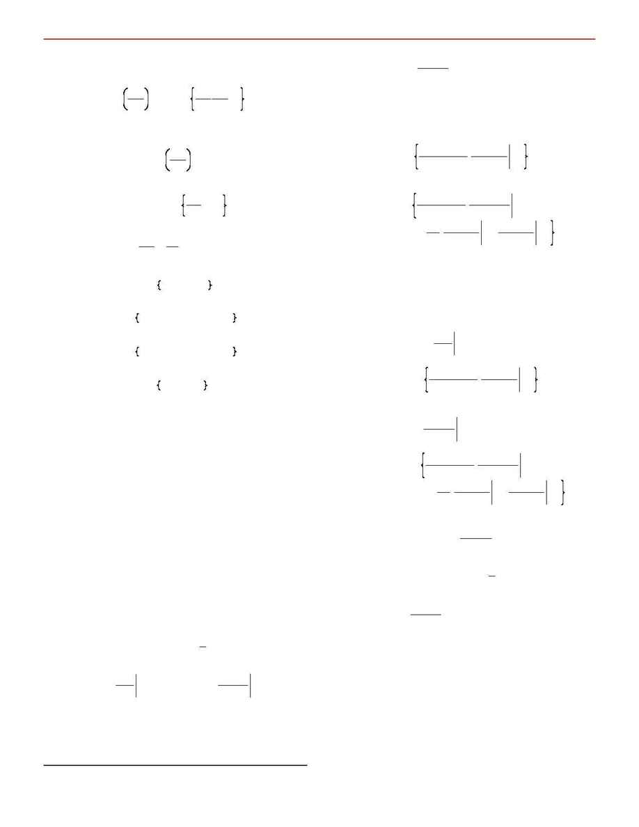
(18), and with a slight abuse of vector notation, we may write
the parameter variance as
(19)
r
a
2
=
¹a
¹y
i
2
r
i
2
i
+
¹a
¹y
i
¹a
¹y
j
r
ij
2
j
i
We will assume that the observational errors are individu-
ally uncorrelated,
. Then we are left with
r
ij
=
0
¼ i ! j
(20)
r
a
2
=
¹a
¹y
i
2
r
i
2
i
Now, from (13) and (8) we have
(21)
a
=
C $ S
=
C $
y
i
r
i
Z(t
i
)
i
Thus,
(22)
¹a
¹y
i
=
1
r
i
C $ Z(t
i
)
Hence, (20) becomes
(23)
r
a
2
=
(C $ Z(t
i
))
2
i
The k
th
component of (23) may be written
(24)
r
a
k
2
=
[C $ Z(t
i
)]
k
[C $ Z(t
i
)]
k
i
Since is symmetric,
C
(25)
r
a
k
2
=
[C $ Z(t
i
)]
k
[Z(t
i
)
$ C]
k
i
Interchange the order of summations:
(26)
r
a
k
2
=
[C $ Z(t
i
) Z(t
i
)
i
$ C]
kk
Using (9), we have
(27)
r
a
k
2
=
[C $ A $ C]
kk
=
[C $ C
-
1
$ C]
kk
=
[C]
kk
which completes the derivation of (14).
4. NONLINEAR PARAMETER ESTIMATION
Consider the condition equations (5). If the model function
is nonlinear in the parameters
then the simple separa-
y(t, a)
tion, eq. (6), which led to the easily-solved normal equations,
(12), is no longer possible. Our goal is to minimize (4) with re-
spect to variation of the model parameters, despite the nonlin-
ear dependence of the model function on the parameters. To
do this, we will adopt an iterative approach.
Let
where are the true (or, more accurately,
a h a~
+
Da,
a~
best) values of the parameters. Assume we start with parameter
values that are reasonably close to the best values. We can
then approximate (4) with a truncated Taylor series:
(28)
x
2
(a) l
x
2
(a~)
-
Da $ B
+
1
2
Da $ M $ Da
where
(29)
B h
-
¹x
2
¹a
a
=
a~
and [M]
ij
h
¹x
2
¹a
i
¹a
j
a
=
a~
Within the paraboloidal approximation (28), the correction
vector
which minimizes
is given by the value for
Da
x
2
(a)
which the parameter correction gradient vanishes:
(30)
¹x
2
(a)
¹Da
l
-
B
+
Da $ M
Hence,
(31)
Da
=
M
-
1
$ B
where we have used the fact that is symmetric. For and
M
B
M
we calculate
(32)
B
=
y
i
-
y(t
i
, a)
r
i
2
¹y(t
i
, a)
¹a
a
=
a~
i
and
(33)
[M]
jk
=
y
i
-
y(t
i
, a)
r
i
2
¹
2
y(t
i
, a)
¹a
j
¹a
k
a
=
a~
-
1
r
i
2
¹y(t
i
, a)
¹a
j
a
=
a~
¹y(t
i
, a)
¹a
k
a
=
a~
i
Unfortunately, although the merit function is unitless, the
elements of eqs. (32) and (33) are not unitless (in general).
This can lead too easily to an ill-conditioned matrix when the
parameters exhibit numerically widely disparate units. There-
fore, following Hessler et al.
5
, let us redefine and
in a
B
M
unitless fashion:
(34)
B
k
h
-
a~
k
¹x
2
¹a
k
a
=
a~
=
a~
k
y
i
-
y(t
i
, a)
r
i
2
¹y(t
i
, a)
¹a
k
a
=
a~
i
and
(35)
[M]
jk
h a~
j
a~
k
¹x
2
¹a
j
¹a
k
a
=
a~
=
a~
j
a~
k
y
i
-
y(t
i
, a)
r
i
2
¹
2
y(t
i
, a)
¹a
j
¹a
k
a
=
a~
-
1
r
i
2
¹y(t
i
, a)
¹a
j
a
=
a~
¹y(t
i
, a)
¹a
k
a
=
a~
i
To keep a unitless form for the merit function, define
(36)
da
k
h a
k
-
a~
k
a~
k
Using (34) and (35), we can rewrite (28) as
(37)
x
2
(a) l
x
2
(a~)
-
da $ B
+
1
2
da $ M $ da
Requiring
(38)
¹x
2
(a)
¹ da
l
-
B
+
da $ M
=
0
we have, finally,
(39)
da
=
M
-
1
$ B
where and are given by (34) and (35). Notice that the
B
M
form of eqs. (39) is identical to that of eqs. (13). The proce-
dure, then, is:
¯ Start with an initial set of values for the parameters.
¯ Calculate the correction via eqs. (39).
¯ Correct the parameter values.
¯ Repeat until the values stop changing significantly.
C
HAPTER
3: T
HE
P
ARAMETER
A
DJUSTMENT
M
ODULE
10
5
J.P. Hessler, D.H. Current, and P.J. Ogren (1996), "A new scheme for calculating weights and describing correlations in nonlinear leastsquares fits", Computers
in Physics 10, 186.
